 Account
 Projects
 Log Out


How to create a grouped bar chart in Excel?

In Excel, creating a grouped bar chart is not that complicated. Many people may find it confusing the first time, but as long as the data is arranged properly, you can make one in just a couple of clicks. The key is to place the rows and columns correctly; otherwise, the chart will look messy. Let’s walk through it step by step.
Prepare the Data Table for the Bar Chart
Preparing the data table is the first and most important step in creating a clear and visually appealing bar chart. Many people get stuck here - - not because they don’t know how to insert a chart, but because the data format is messy, and the result ends up distorted.
Before starting, let’s ask: is the data suitable for a bar chart? Not all data works well in this format. If the data is better suited for a line chart or pie chart, forcing it into a bar chart will only make it harder to read. We covered this in a dedicated article: Where Bar Chart Is Used?. If you haven’t read it yet, we recommend checking it out.
Once the data is confirmed to be suitable, it can be prepared in a simple format:
- Put the time or category labels in the first column - for example, months, quarters, or years.
- Put the group names in the first row - for example, Smartphone, Laptop, or Tablet.
- Fill in the values in the middle cells, which are the actual numbers corresponding to each category and time.
Like this:
| Date | Smartphone | Laptop | Tablet | Smartwatch | Headphones | Speaker | Keyboard |
|---|---|---|---|---|---|---|---|
| January | 4200 | 3100 | 1800 | 900 | 2600 | 1400 | 1200 |
| February | 4500 | 3300 | 1700 | 1100 | 2800 | 1300 | 1300 |
| March | 4900 | 3500 | 2000 | 1300 | 3000 | 1800 | 1400 |
| April | 5100 | 3700 | 2200 | 1500 | 3100 | 1900 | 1500 |
By default, when we select the data in Excel and insert a grouped bar chart, Excel will treat the columns as groups. In this case, it will generate 7 groups, each containing 4 bars (January, February, March, April).
Insert a Grouped Bar Chart in Excel
Once the table is ready, just two simple steps are needed to create a grouped bar chart.
Step 1: Select the Data Range
In this example, simply use the mouse to select the entire table. In some cases, only part of the table may be needed - just select the portion you want.
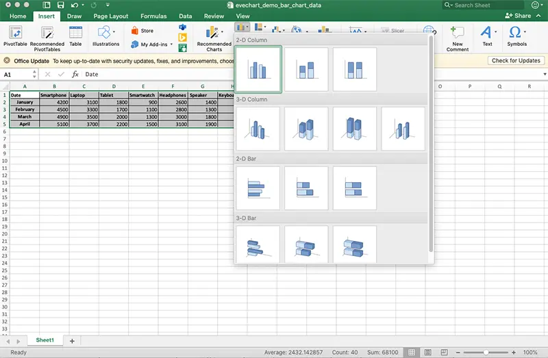
Step 2: Insert the Chart
Click “Insert”, then choose the first Grouped Column Chart from the bar chart options.
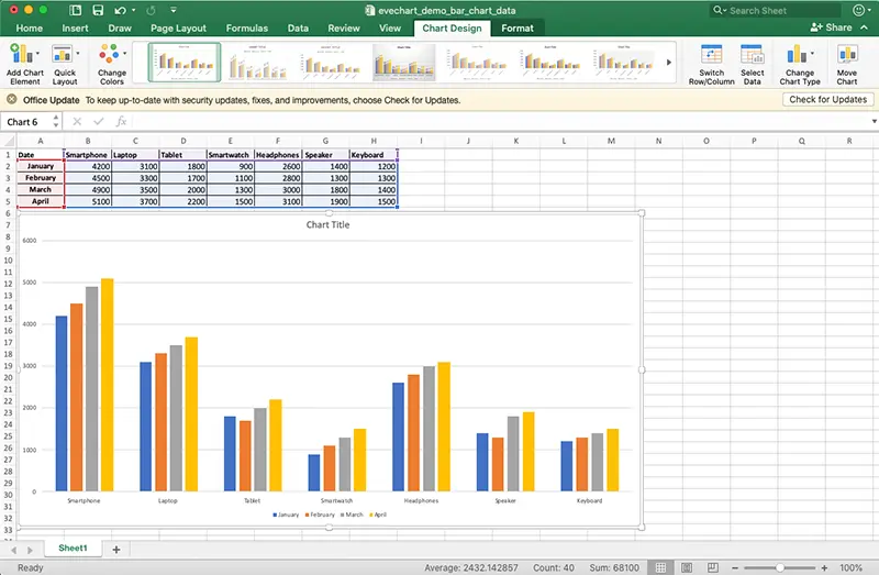
That’s it - two simple steps and the grouped bar chart is ready. Next, let’s make it a bit more polished.
Beautify the Bar Chart
The default grouped bar chart in Excel works, but let’s be honest - it doesn’t look great. It’s fine for personal review, but in a report it often looks plain.
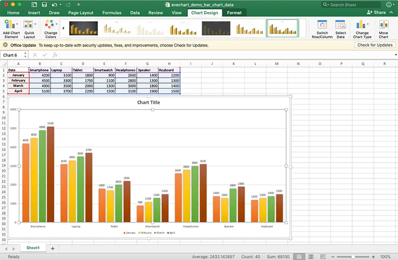
In Excel, a few simple adjustments can help:
- Change the color scheme to make the series easier to distinguish.
- Adjust the chart style - for example, remove gray gridlines or modify the layout.
- Add a title that’s short and clear, so anyone knows immediately what the chart is about.
These are all very simple operations: just click the color or style buttons in the toolbar, and they apply instantly.
Export and Save the Bar Chart
Once the chart is ready, the next step is usually to use it - either in a PowerPoint presentation, a Word report, or as an image.
In Excel, the two most common ways are:
- Copy & Paste: Copy the chart and paste it into PowerPoint or Word.
- Save as Picture: Right-click the chart, choose “Save as Picture,” and you’ll get a standalone image.
The problem is that Excel’s exported images are usually not very sharp. They look fine on a screen, but once printed or enlarged in a presentation, they turn blurry. That’s one of the most common complaints: Excel charts don’t look “professional enough.”
If high-resolution images or formats like SVG are needed for lossless scaling, Excel falls short. This is where EveChart comes in - it can export high-resolution PNGs and SVGs in one click, saving a lot of hassle.
A More Efficient Choice: Use EveChart Professional Chart Generator
To be fair, Excel can create grouped bar charts for basic needs, but anyone who has used it knows there are some pain points:
- Limited export quality: Enlarged or printed images look blurry, not professional.
- Data manipulation is clumsy: Hiding a few columns of data usually requires rebuilding or adjusting the chart manually.
- Switching views is inconvenient: Swapping the X and Y axes or making the chart horizontal requires multiple manual adjustments.
Put together, these issues make many people feel that Excel charts are “usable, but not user-friendly.”
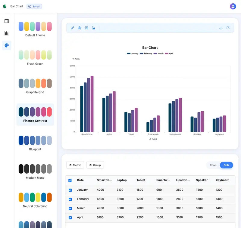
With EveChart, all of these pain points are solved with one click:
- Export high-resolution PNG and SVG images, perfect for PowerPoint or academic papers.
- Instantly control what data is displayed by simply checking rows or columns, no need to rebuild the chart.
- One-click swap X and Y axes, and one-click horizontal chart layout - fast and effortless.
Best of all, EveChart can be tried for free right now - no installation, no complicated setup. 👉 Try EveChart Now
And for more chart usage tips, check out: Bar Chart Quick Start Guide, which will help quickly master the most common use cases.


 EN
EN